Boundary design mlb with single fluidic lane adjacent to sidewalls

import matplotlib.pyplot as plt
import numpy as np

from mnflow.mfda.cad.dld.theme.block import DLD

dld = DLD(
    d_c=10.0,
    Np=40,
    # boundary
    boundary_treatment='mlb',
    #
    rotation_angle_deg_before_array=90,
    # image
    opt_save_image=True,
    img_dpu=.4,
)

----------------------------------------
core.DLD___Np:40_Nw:8_gap_w:41.962_pitch_w:83.925_gap_a:41.962_pitch_a:83.925_height:167.850_boundary_treatment:mlb
block.DLD___num_unit:9_opt_mirror:False_array_counts:[1, 1]_opt_mirror_before_array:[False, False]
----------------------------------------
{'Np': 40,
 'Nw': 8,
 'area': 27242538.116219997,
 'bb': [(-30170.993, -218.202), (41.962, 683.482)],
 'count of 1D arrays of core.DLD': 1,
 'd_c': 9.999999999999998,
 'lx': 30212.954999999998,
 'ly': 901.684,
 'performance': {'Flow rate @ 1 bar/area (micro-liter/min/mm-sq)': 86.14517084708385,
                 'die area (mm-sq)': 27.242538116219997,
                 'gap over crit. dia.': 4.1962442597075205,
                 'volumetric flow rate at 1 bar (micro-liter/min)': 2346.8131003299654},
 'resistance (Pa.sec/m^3)': 2556658644506.6255,
 'volumetric flow rate at 1 bar (m^3/sec)': 3.911355167216609e-08,
 'volumetric flow rate at 1 bar (milli-liter/hr)': 140.80878601979794}

Output layout:

Visualization of gap profiles

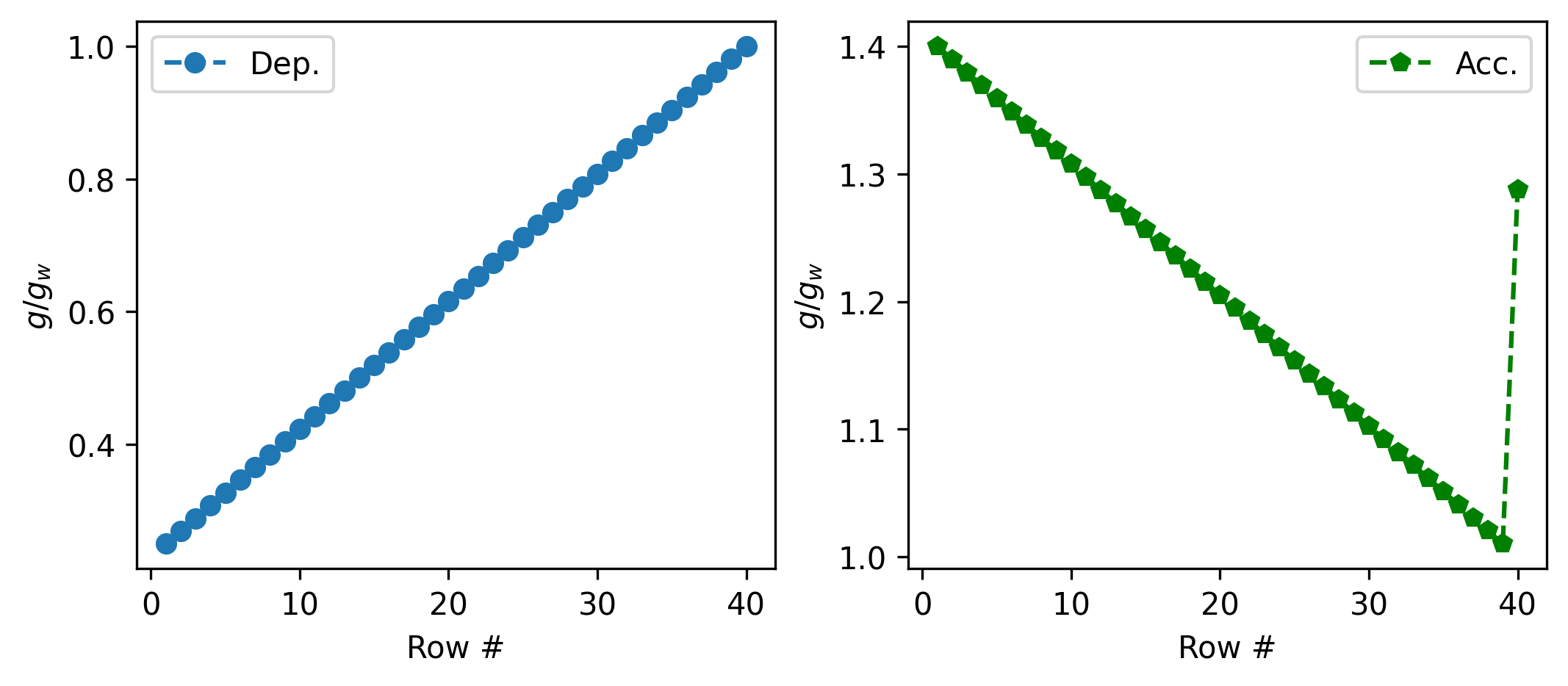
Here is how dimensionless gap profiles look like for depletion and accumulation sidewalls:

Np=dld.Np
gap_a=dld.gap_a
gap_w=dld.gap_w
phi=dld.phi
boundary_gaps=dld.get_boundary_gaps()

dep_gap=np.array(boundary_gaps['dep'][:,:-1]).flatten()
acc_gap=np.array(boundary_gaps['acc']).flatten()
if boundary_gaps['acc_usm_gap_a_widening'] is None:
    boundary_gaps['acc_usm_gap_a_widening']=0
acc_Nth_lat_gap=boundary_gaps['acc_usm_gap_a_widening']+gap_a

fig, ax=plt.subplots(1,2,figsize=(7,3),dpi=300, layout="constrained")
ax[0].plot(np.arange(1,Np+1), dep_gap[::-1]/gap_w, '--o', label="Dep.")
ax[1].plot(np.arange(1,Np+1), acc_gap[::-1]/gap_w, '--gp', label="Acc.")
ax[0].set_xlabel('Row #')
ax[1].set_xlabel('Row #')
ax[0].set_ylabel(r'$g/g_w$')
ax[1].set_ylabel(r'$g/g_w$')
ax[0].legend()
ax[1].legend()
plt.show()

And, values of important parameters and variables:

print("Np: ", Np)
print("gap_w: ", gap_w)
print("phi: ", phi)
print('gap dep: ', dep_gap)
print('gap acc: ', acc_gap)
print('gap acc widening -- Nth row, lat: ', boundary_gaps['acc_usm_gap_a_widening'])
print('gap acc -- Nth row, lat: ', acc_Nth_lat_gap)

Np:  40
gap_w:  41.962442597075196
phi:  1
gap dep:  [41.9624426  41.15541286 40.34838313 39.5413534  38.73432367 37.92729393
 37.1202642  36.31323447 35.50620473 34.699175   33.89214527 33.08511553
 32.2780858  31.47105607 30.66402634 29.8569966  29.04996687 28.24293714
 27.4359074  26.62887767 25.82184794 25.01481821 24.20778847 23.40075874
 22.59372901 21.78669927 20.97966954 20.17263981 19.36561007 18.55858034
 17.75155061 16.94452088 16.13749114 15.33046141 14.52343168 13.71640194
 12.90937221 12.10234248 11.29531275 10.48828301]
gap acc:  [54.04571856 42.39284855 42.82325451 43.25366046 43.68406642 44.11447238
 44.54487833 44.97528429 45.40569024 45.8360962  46.26650215 46.69690811
 47.12731407 47.55772002 47.98812598 48.41853193 48.84893789 49.27934384
 49.7097498  50.14015576 50.57056171 51.00096767 51.43137362 51.86177958
 52.29218553 52.72259149 53.15299745 53.5834034  54.01380936 54.44421531
 54.87462127 55.30502722 55.73543318 56.16583914 56.59624509 57.02665105
 57.457057   57.88746296 58.31786891 58.74827487]
gap acc widening -- Nth row, lat:  12.083275959679746
gap acc -- Nth row, lat:  54.04571855675494