Boundary profile pow without pressure balance

import matplotlib.pyplot as plt
import numpy as np

from mnflow.mfda.cad.dld.theme.block import DLD

dld = DLD(
    d_c=10.0,
    Np=10,
    # boundary
    boundary_treatment='pow',
    opt_acc_balance_pressure=False,
    #
    rotation_angle_deg_before_array=90,
    # image
    opt_save_image=True,
    img_dpu=5,
)

----------------------------------------
core.DLD___Np:10_Nw:8_gap_w:21.571_pitch_w:43.142_gap_a:21.571_pitch_a:43.142_height:86.284_boundary_treatment:pow
block.DLD___num_unit:9_opt_mirror:False_array_counts:[1, 1]_opt_mirror_before_array:[False, False]
----------------------------------------
{'Np': 10,
 'Nw': 8,
 'area': 1775013.340104,
 'bb': [(-3861.227, -112.011), (21.571, 345.137)],
 'count of 1D arrays of core.DLD': 1,
 'd_c': 9.999999999999998,
 'lx': 3882.798,
 'ly': 457.148,
 'performance': {'Flow rate @ 1 bar/area (micro-liter/min/mm-sq)': 718.4068858355761,
                 'die area (mm-sq)': 1.7750133401039998,
                 'gap over crit. dia.': 2.1571083717157262,
                 'volumetric flow rate at 1 bar (micro-liter/min)': 1275.1818059807188},
 'resistance (Pa.sec/m^3)': 4705211423076.657,
 'volumetric flow rate at 1 bar (m^3/sec)': 2.1253030099678647e-08,
 'volumetric flow rate at 1 bar (milli-liter/hr)': 76.51090835884312}

/usr/bin/xdg-open: 882: www-browser: not found
/usr/bin/xdg-open: 882: links2: not found
/usr/bin/xdg-open: 882: elinks: not found
/usr/bin/xdg-open: 882: links: not found
/usr/bin/xdg-open: 882: lynx: not found
/usr/bin/xdg-open: 882: w3m: not found
xdg-open: no method available for opening '/tmp/tmpm5s1xqpl.PNG'

Output layout:

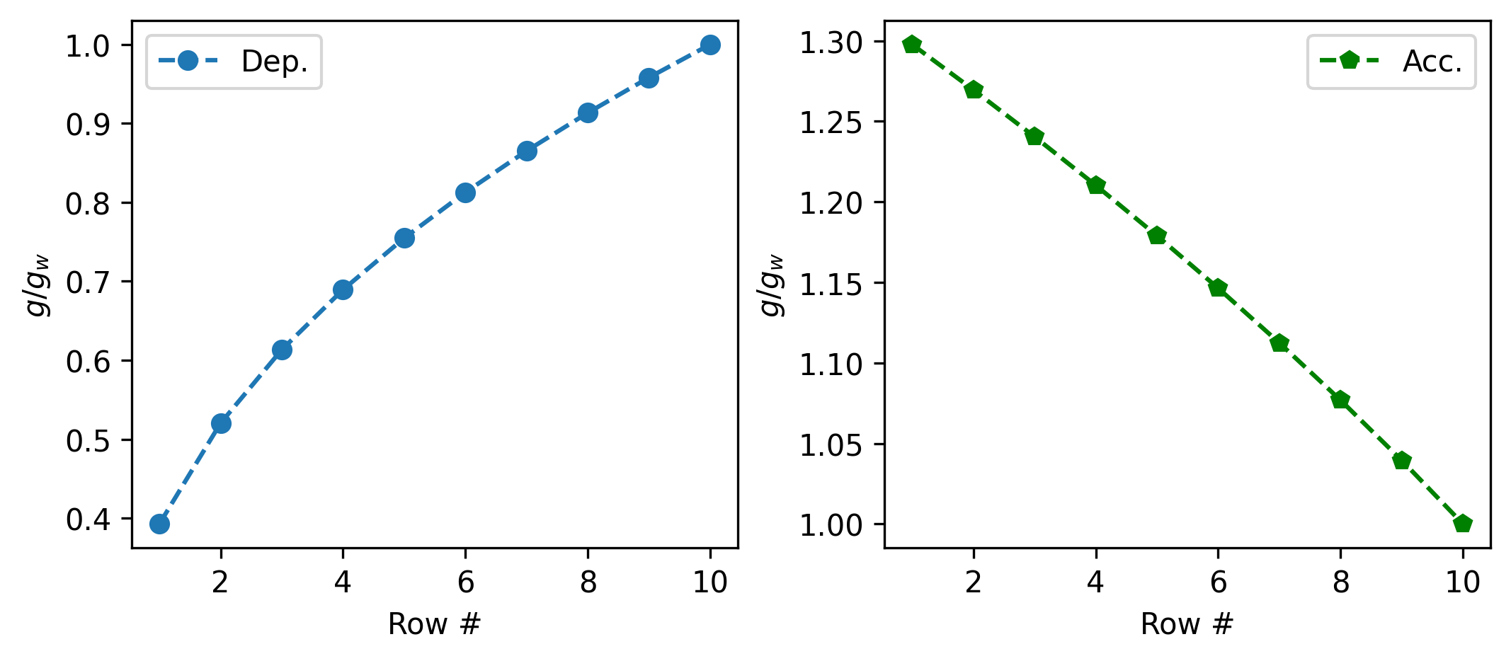
Visualization of gap profiles

Here is how dimensionless gap profiles look like for depletion and accumulation sidewalls:

Np=dld.Np
gap_a=dld.gap_a
gap_w=dld.gap_w
phi=dld.phi
boundary_gaps=dld.get_boundary_gaps()

dep_gap=np.array(boundary_gaps['dep'][:,:-1]).flatten()
acc_gap=np.array(boundary_gaps['acc']).flatten()
if boundary_gaps['acc_usm_gap_a_widening'] is None:
    boundary_gaps['acc_usm_gap_a_widening']=0
acc_Nth_lat_gap=boundary_gaps['acc_usm_gap_a_widening']+gap_a

fig, ax=plt.subplots(1,2,figsize=(7,3),dpi=300, layout="constrained")
ax[0].plot(np.arange(1,Np+1), dep_gap[::-1]/gap_w, '--o', label="Dep.")
ax[1].plot(np.arange(1,Np+1), acc_gap[::-1]/gap_w, '--gp', label="Acc.")
ax[0].set_xlabel('Row #')
ax[1].set_xlabel('Row #')
ax[0].set_ylabel(r'$g/g_w$')
ax[1].set_ylabel(r'$g/g_w$')
ax[0].legend()
ax[1].legend()
plt.show()

And, values of important parameters and variables:

print("Np: ", Np)
print("gap_w: ", gap_w)
print("phi: ", phi)
print('gap dep: ', dep_gap)
print('gap acc: ', acc_gap)
print('gap acc widening -- Nth row, lat: ', boundary_gaps['acc_usm_gap_a_widening'])
print('gap acc -- Nth row, lat: ', acc_Nth_lat_gap)

Np:  10
gap_w:  21.571083717157258
phi:  1
gap dep:  [21.57108372 20.66778878 19.70269495 18.66295397 17.53070535 16.27987617
 14.86978764 13.23056904 11.22235232  8.46960258]
gap acc:  [21.57108372 22.42217636 23.22845142 23.99573091 24.72869807 25.43118448
 26.1063707  26.75693014 27.38513471 27.99293374]
gap acc widening -- Nth row, lat:  0
gap acc -- Nth row, lat:  21.571083717157258