Boundary profile 3d with pressure balance
import matplotlib.pyplot as plt
import numpy as np

from mnflow.mfda.cad.dld.theme.block import DLD
dld = DLD(
    d_c=10.0,
    Np=10,
    # boundary
    boundary_treatment='3d',
    #
    rotation_angle_deg_before_array=90,
    # image
    opt_save_image=True,
    img_dpu=5,
)
----------------------------------------
core.DLD___Np:10_Nw:8_gap_w:21.571_pitch_w:43.142_gap_a:21.571_pitch_a:43.142_height:86.284_boundary_treatment:3d
block.DLD___num_unit:9_opt_mirror:False_array_counts:[1, 1]_opt_mirror_before_array:[False, False]
----------------------------------------
{'Np': 10,
 'Nw': 8,
 'area': 1797556.865292,
 'bb': [(-3861.227, -112.337), (21.571, 350.617)],
 'count of 1D arrays of core.DLD': 1,
 'd_c': 9.999999999999998,
 'lx': 3882.798,
 'ly': 462.954,
 'performance': {'Flow rate @ 1 bar/area (micro-liter/min/mm-sq)': 709.397199389058,
                 'die area (mm-sq)': 1.7975568652919998,
                 'gap over crit. dia.': 2.1571083717157262,
                 'volumetric flow rate at 1 bar (micro-liter/min)': 1275.1818059807188},
 'resistance (Pa.sec/m^3)': 4705211423076.657,
 'volumetric flow rate at 1 bar (m^3/sec)': 2.1253030099678647e-08,
 'volumetric flow rate at 1 bar (milli-liter/hr)': 76.51090835884312}
/usr/bin/xdg-open: 882: www-browser: not found
/usr/bin/xdg-open: 882: links2: not found
/usr/bin/xdg-open: 882: elinks: not found
/usr/bin/xdg-open: 882: links: not found
/usr/bin/xdg-open: 882: lynx: not found
/usr/bin/xdg-open: 882: w3m: not found
xdg-open: no method available for opening '/tmp/tmpx_d4j3i4.PNG'
Output layout:

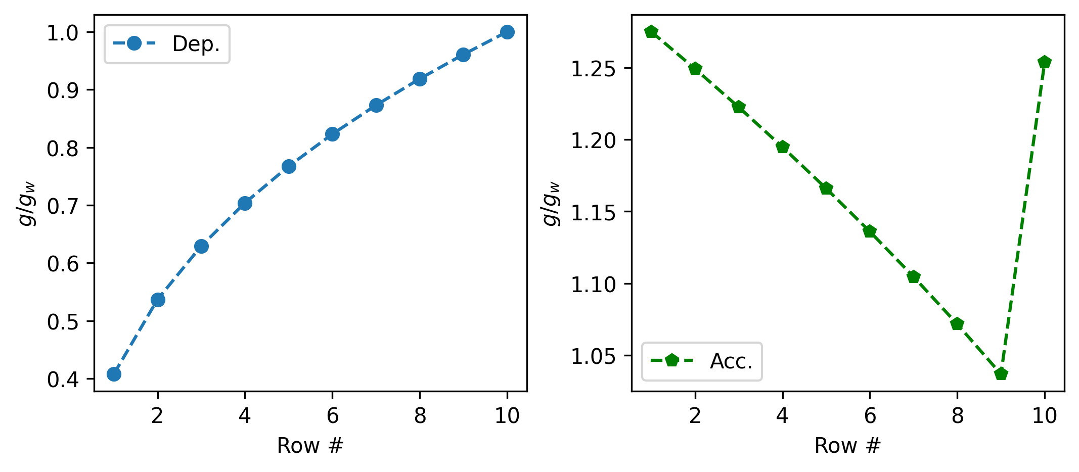
Visualization of gap profiles
Here is how dimensionless gap profiles look like for depletion and accumulation sidewalls:
Np=dld.Np
gap_a=dld.gap_a
gap_w=dld.gap_w
phi=dld.phi
boundary_gaps=dld.get_boundary_gaps()

dep_gap=np.array(boundary_gaps['dep'][:,:-1]).flatten()
acc_gap=np.array(boundary_gaps['acc']).flatten()
if boundary_gaps['acc_usm_gap_a_widening'] is None:
    boundary_gaps['acc_usm_gap_a_widening']=0
acc_Nth_lat_gap=boundary_gaps['acc_usm_gap_a_widening']+gap_a

fig, ax=plt.subplots(1,2,figsize=(7,3),dpi=300, layout="constrained")
ax[0].plot(np.arange(1,Np+1), dep_gap[::-1]/gap_w, '--o', label="Dep.")
ax[1].plot(np.arange(1,Np+1), acc_gap[::-1]/gap_w, '--gp', label="Acc.")
ax[0].set_xlabel('Row #')
ax[1].set_xlabel('Row #')
ax[0].set_ylabel(r'$g/g_w$')
ax[1].set_ylabel(r'$g/g_w$')
ax[0].legend()
ax[1].legend()
plt.show()
And, values of important parameters and variables:
print("Np: ", Np)
print("gap_w: ", gap_w)
print("phi: ", phi)
print('gap dep: ', dep_gap)
print('gap acc: ', acc_gap)
print('gap acc widening -- Nth row, lat: ', boundary_gaps['acc_usm_gap_a_widening'])
print('gap acc -- Nth row, lat: ', acc_Nth_lat_gap)
Np:  10
gap_w:  21.571083717157258
phi:  1
gap dep:  [21.57108372 20.72435036 19.81536111 18.83064117 17.75137758 16.54999034
 15.18327877 13.57679303 11.58120825  8.79622382]
gap acc:  [27.05042239 22.36558198 23.11552308 23.82693461 24.50464505 25.15258884
 25.77401901 26.37165941 26.9478161  27.50446055]
gap acc widening -- Nth row, lat:  5.479338675468252
gap acc -- Nth row, lat:  27.05042239262551